Introduction to the XY Model

In the previous post, [[link]], we talked about our realization of the XY-model, tilted, smectic liquid crystals. In this post, we’ll go into a little more detail about the XY-model, and how it ties in with machine learning.

The XY model is a simple model to describe. First, picture a grid.

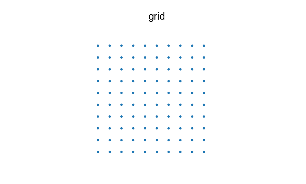xy model grid a simple grid

Now, at every point on the grid, we put a little arrow, denoting the spin at that location.

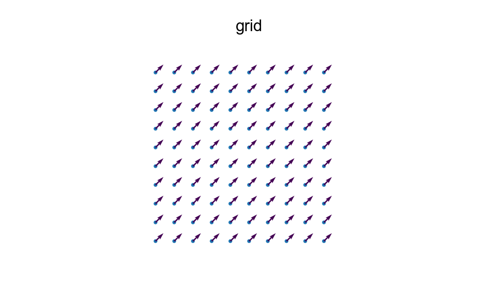xy model grid with spin a simple grid with spins

That is it. This is the foundation of the XY model. It is admittedly pretty boring though. The next step is to have these spins interact with themselves. A natural choice for interaction is that the spins want to be aligned (ferroelectric ordering). We also demand that the interaction is hyper-local: every spin can only interact with its nearest neighbors. The simplest mathematical realization of this is the interaction potential:

$H = \sum_{i,j}^N s_i \cdot s_j = \sum_{i,j}^N \cos(\theta_i -\theta_j)$

However, because all the spins are pointing in the same direction, this system has the lowest energy possible, so it’s not very exciting. We can randomize the system, so that every point has a spin at some random direction.

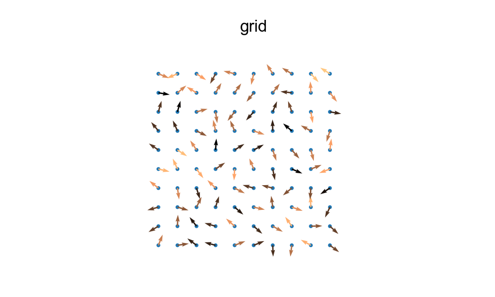xy model grid with random spins a simple realization of the XY model with random intial state

We can also plot the energy of the system: at every grid site, we can solve for what the interaction energy is:

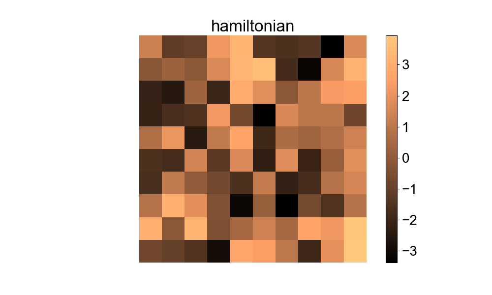xy model hamiltonian The hamiltonian of our random XY model

You’ll notice, I was also sneaky and colour-coded the spins in the XY-grid picture, where the colour reflects how much interaction energy they have.

Vortices in the XY-Model

One of the main things that is interesting about the XY model is that it supports vortices. Vortices are easier to talk about in the continuous version of the xy model. So imagine we take our grid, and take the limit of lattice spacing to zero– boom, we’re now in a continuous space[:1]. How does our interaction energy change? Ask any physicist a question and they’ll suggest Taylor expansion, so that’s what we’ll do. But I don’t want to write out all the tex, so you can trust me that in a continuous space, our interaction energy (to first order anyway) becomes: $h = \left( \nabla \theta\ \right )^2.$

Now, we’re trying to get to a pithy explanation of what a vortex is. Taking a very broad outlook, a vortex is a certain spatial configuration of spins. Armed now with our Hamiltonian, we can begin looking at what spatial configurations are allowed by the XY interaction. To do that, we’ll do the usually physics sleight of hand by pretending that $h$ is a free-energy, and set the functional derivative equal to zero to find the minimum free-energy state. Doing that, we get: $\frac{\delta h}{\delta \theta(x,y)} \propto \nabla^2 \theta(x,y) = 0$

Oh, it’s a Laplacian. That is comforting, now we can call Papa Maxwell and get him to solve this without breaking a sweat. Without boundary conditions, the solution to this would just be a uniform field (everything aligned). But we have an additional, subtle restriction¹ on our $\theta(x,y)$ field. It is not a scalar field, so we can’t use the most familiar solution to Laplace’s equation: the point-charge potential.

We are able to pretend it is a scalar field because of two things:

We are in 2D, so we can encode any 2D vector as a complex function, $\vec{v} \rightarrow r\exp(i\phi)$ .
The magnitude of our spin field is constant ( $r$ doesn’t change with spatial transformations). This just means that every spin on our grid has a length of 1.

This allows us to hide away the fact that every spin that sits on our grid is actually a 2D vector of magnitude one.

But Maxwell does give us tools for dealing with Laplace’s equation with vector fields, we just have to turn to magnitism rather than electrostatics. The solution we are looking for is the same one that describes the vector-potential field around a current-carrying wire.

$\theta = \pm \phi + \theta_0$

And the same way you can get information about the ‘current’ strength by doing a line integral of the vector-potential around the wire, you can get information about the defect strength by doing a line integral around the defect. Line integrals become a lot more ambiguous on a grid, where you only have 4 segments to add up, but the following is a general algorithm for classifying defects.

For our grid, a vortex is any plaquette where, when you walk around the perimeter in a counter-clock wise direction, adding up the spin at every grid point as you go, you’ll get a value whose magnitude is greater than 2π. The sign of the value you get tells you the charge of the defect. I’ve shown a picture below with a plus and a minus defect. Notice, once we actually render the spins, they are a true vector field– not a scalar field as you might guess!

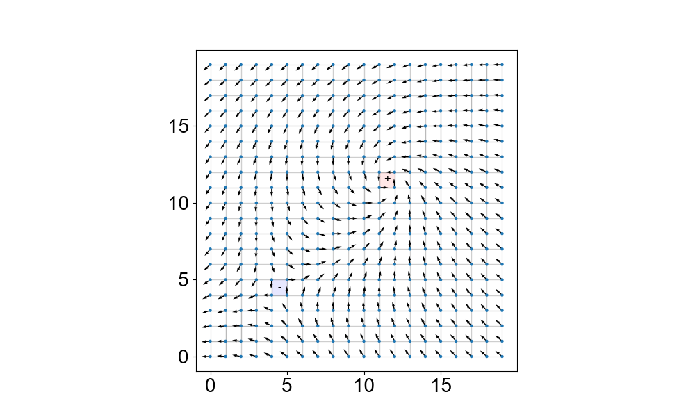xy model with labeled defects The XY model with plus and minus vortices

I ran out of time today, but next I’ll discuss what these would actually look like under a microscope.

So, hopefully you get the flavour of what the XY model is, and how it has a rich enough mathematical structure to support vortices!

See you next time.

I’m pretty sure about this, but I haven’t worked it out in detail. ↩

PREVIOUSUsing Deep Learning Algorithms for Defect Detection

NEXTEnhancing Simulation Data for use in Machine Learning