Algorithms
A great deal of research has been performed on applying deep learning to object detection tasks. The resulting methods have proved to be quicker and more accurate than traditional computer vision techniques, however, adoption of these algorithms for laboratory usage has lagged due to the difficulty in acquiring the large, labeled datasets necessary for training neural networks. We will be attempting to determine the efficacy of generating labeled training data from a simulation and using it to detect defects in real-world data. Ideally, we would also like to create a simple pipeline allowing the detection of other objects to be quickly automated.
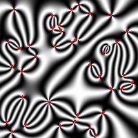
For reference, the images we are attempting to annotate look like the one below. Defects are the points marked by red dots.
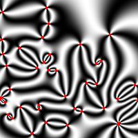 Sample Defect Image
The three most popular algorithms for object detection are RCNN (and its successors), Single Shot Detectors (SSD), and YOLO. Although all three approaches make use of deep neural networks, their methods of finding bounding boxes differ greatly. It is important to understand these differences, so I will provide a brief summary of each. R-CNN – Region Convolutional Neural network. The most modern version is known as Faster R-CNN. This algorithm uses a search function to find potential candidate objects to run object recognition on. Slower, but accurate. Unfortunately, since this algorithm depends on only running the neural network on likely object candidates detected in an untrainable search algorithm, it will most likely perform poorly at detecting objects that don’t fit traditional ideas of what constitutes an object.
SSD- Single Shot (multi-box) Detector. This algorithm works by creating multiple default bounding boxes over the entirety of an image. A neural network scores the bounding boxes and provides a prediction for how to adjust the regions to maximize a high class. Faster than R-CNN, but slightly less accurate.
YOLO – You Only Look Once. The input image is initially divided into a grid. Each cell in the grid is used to predict five bounding boxes. A classifier is run for each predicted bounding box, and outcomes with high certainty scores are returned as objects. This is the fastest of the three algorithms, although slightly less accurate in general. However, since the features we are looking at aren’t typical objects this method is likely to work better than R-CNN.
Since we will be attempting to detect defects, which do not look like the ordinary definition of an object (see above image), R-CNN would make a poor choice. Both SSD and YOLO are likely to produce good results. YOLO has the advantage of having a highly accessible implementation known as darkflow, which uses the python TensorFlow library on the backend. This a major advantage when considering accessibility for scientists or industrial users who may need to make their own modifications, as python is a much more readable and easier to understand language than other languages commonly used for deep learning algorithms.
Darkflow
The original darkflow repository can be found here https://github.com/thtrieu/darkflow The repository for our modified code can be found here https://github.com/mlfilms/defectTracker Our code includes scripts for simplifying the process of training and running the algorithm. To make a model, you will also need the default weights file to train from, which is located at https://drive.google.com/drive/u/2/folders/1c_xrWVKNBuqZUwXGvv_MBamOHNa1wBKy along with other trained models. Download the yolo.weights file and place it in a bin folder.
The readme included in the repo explains how to use the system in detail, and includes instructions on installing dependencies.
Inside the darkflow folder are three scripts that make running training, running, and validating the model easier. trainFlow.py uses annotations and images to train a model. Adjust the batch size or GPU usage number if you run into memory errors. runFlowPB.py loads a model from the .pb and .meta files generated when a model is finished training. The images in the specified directory will be analyzed and marked images will be output, along with JSON files containing the detections. Finally, validation .py makes use of code from https://github.com/Cartucho/mAP to evaluate how well a trained model performs
Also included are scripts for generating simple training data datasets consisting of images with circles. As a first order test, this simulated data was used to evaluate the effectiveness of YOLO for detecting circles when compared with a common, non-ML algorithm, the circular Hough transform. Although both methods were able to properly label almost all circles in clear images, YOLO showed superiority at detecting circles in noisy data, yielding a mAP score of around 80% when the Hough transform failed to detect any circles.
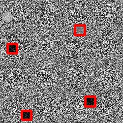 The YOLO detections in noisy data. The circular hough transform failed to detect any circles in this data.
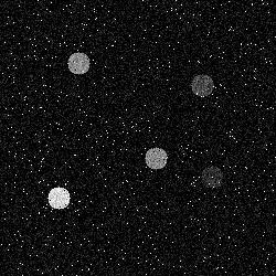 Clear images of circles. Both the circular hough transform and YOLO were able to detect almost all images in this dataset.
This demonstrates the viability of YOLO at providing superior performance detecting objects in imperfect or noisy data, as is often necessary for real scenarios.
Training the model took around 45 minutes on a GTX 1080 GPU, and the final model was able to label 200 images in about 25 seconds, demonstrating the viability of training and using darkflow without the need for specialized hardware.
The system can be set up on a windows computer running anaconda in three commands and can be retrained, ran, and validated with easily with three scripts written to simplify the process.
This allowed a new model to be quickly trained and run on simulated data for defects. The defect simulation and physical significance will be explained in detail in a later post. The initial results are promising on both noisy and clean data.
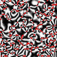 Noisy, crowded simulated defect data. The red markers are all the defect detections from YOLO. Although almost no defects are missed, several false detections exist.
 .
Clean simulated defect data. The trained model was able to accurately label all defects with few mistakes.
The next step is to assess the viability of the models trained on simulated data at detecting defects in experimental data.