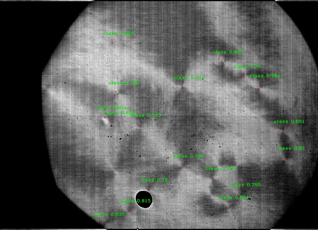
Although we are able to generate perfectly annotated simulation data, the simulation data doesn’t necessarily represent the data we see in actual experiments. This causes issues when trying to train a darkflow model with simulation data to detect defects in the experimental data. The model will not learn to deal with issues such as noise, low contrast, brightness changes, and blurring from the perfect images of our simulation outputs. Thus, we need to process the simulation images to add in the various imperfections present in experimental data. The experimental images will also need to be processed to standardize their appearance regardless of inconsistencies made during data collection.
Image Data Standardization
The brightness and contrast of the experimental images can vary based on factors such as the illumination, polarizer angle and film thickness. In order to make the image data look as similar as possible between runs, we standardize the mean and variances of the images. This is done by subtracting the mean pixel intensity of the image from each pixel, and then dividing that quantity by six times the standard deviation of the pixel intensity values. Adding 0.5 yields pixel intensity values centered around 0.5. In equation form,
This standardization ensures a similar dynamic range and brightness regardless of the specific lighting in an experiment. A similar standardization is applied to the simulation data, to give the simulation and experimental data similar dynamic ranges. However, the simulation has the offset (mean) and standard deviation slightly randomized in order to help the model learn to identify defects in a wider contrast range.
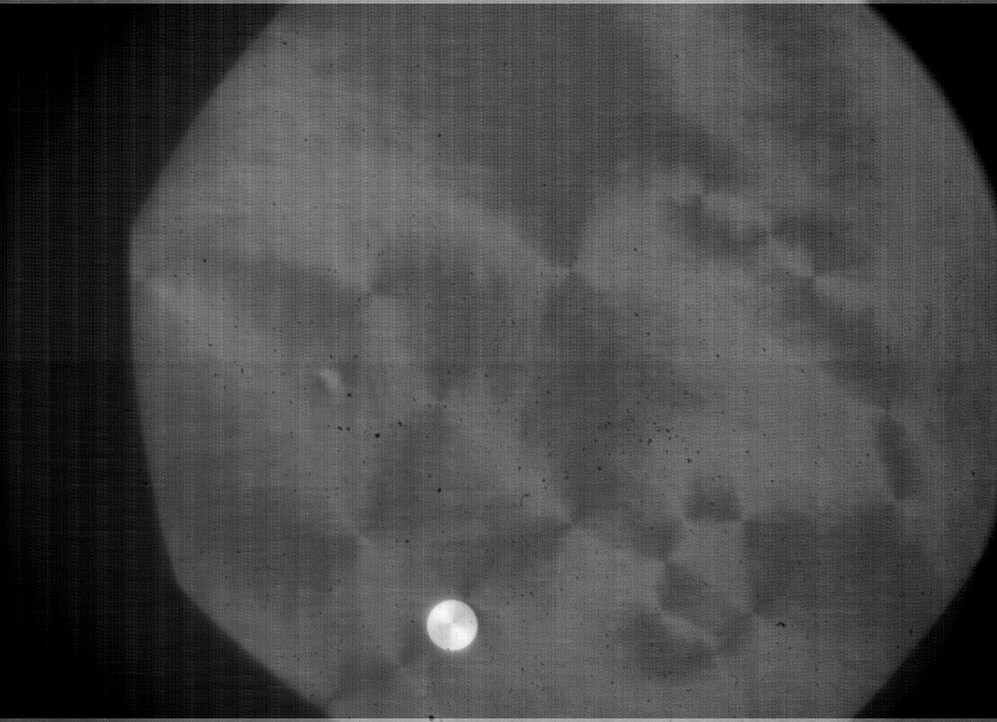 Experimental image before standardization
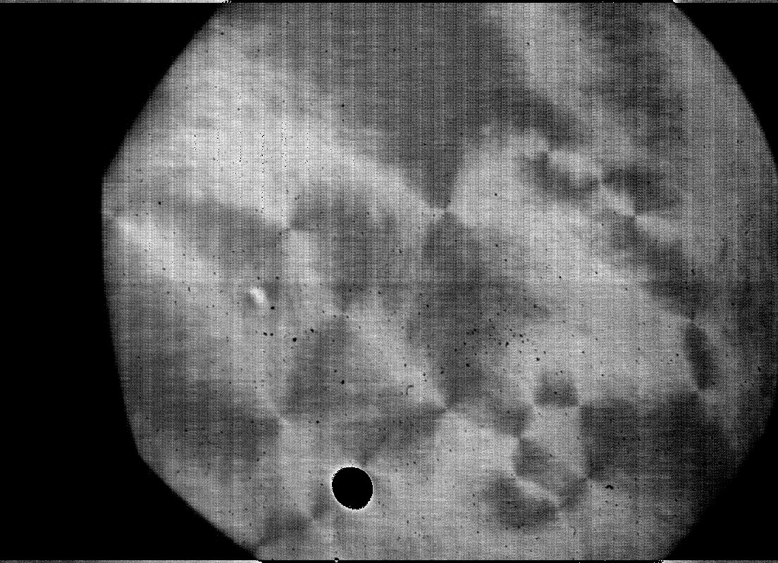 Experimental image after standardization
Accounting For Traditional Experimental Noise
Although it is important to make the experimental data as consistent as possible, it is equally important to make the training data as inconsistent as possible. If you train the model only with images containing distinct intensity levels and gradients, the model will learn to rely on those specific patterns to identify defects. Instead, we wish to make the model as robust as possible by training it on images with a variety of different lighting levels, contrasts, and visual artifacts in order to force the model to recognize the more abstract pattern of a defect. This will result in a model that is able to identify a wider variety of defects in a much larger set of experimental conditions.
 Typical experimental image after standardization
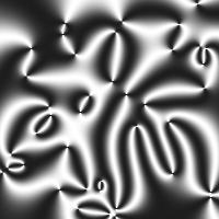 Typical simulated image after standardization
To this end, we add several aberrations to the simulated data.
Gaussian blurring is a simple filter designed to lower the sharpness of an image. When a Gaussian filter is applied, each pixel in an image has its value changed to a weighted mean of the pixels around it. Simulated defect images are very sharp as there is very little inaccuracy when generating the images. However, in experimental images, there are several factors that can result in reduced sharpness. Simple camera inaccuracies are always a factor along with microscopes being slightly out of focus. Light can also be slightly distorted when passing through lenses or being reflected off a surface. The end result is that a machine learning model needs to be trained to identify objects in a variety of blurriness levels, which is why we apply a 2D Gaussian filter to the image with a randomized sigma parameter to the simulated images.
Although we attempt to standardize our experimental images based on the mean and standard deviation of the image data, variations in light and dark regions can skew the standardization process. The presence of especially bright regions, due to inconsistencies in the films layer counts known as islands, can significantly skew the standard deviation of the image. This can wash out the contrast in defect patterns. Thus, the model needs to recognize defects regardless of the particular contrast or brightness levels in an image. To this end, we randomize the standardization process for simulation images. Instead of giving the images a set mean of 0.5 and a dynamic range of 6 standard deviations, the images have their dynamic range and mean set randomly, allowing the model to adapt to a wider range of images.
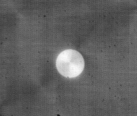 Bright island in a film
When performing photomicroscopy, you often get the boundaries of the microscope apperature in the images, which appear as a sharp transition to dark. Furthermore, older cameras will have distinct brightness shifts partway through the image (visible in the experimental images above on this post). These can be caused due to manufacturing inaccuracies or sensor degradation over time. The early version of the machine learning model would place detections along these boundaries, as it associated areas of quick shifts from light to dark as defects. To help the model learn to ignore such boundaries, similar shifts were added to the simulation images. Each simulation image was broken into four randomized quadrants, with each quadrant having its brightness randomly increased or decreased. After training on this new simulated data, the model successfully learned not to recognize random boundaries as defects.
Smart Noise
The high framerate, light reflecting setup and cross-polarizing conditions of our experimental setup mandate that we collect data with a high ISO and low exposure time. These conditions consequently lead to a low signal size, with the image being predominantly low light levels and low contrast. As such, read noise becomes a major concern over the dim background image.
Read noise is noise generated by the electronics of a camera when data is read from the CCD to memory of the camera. Since read noise is generated when the data is read from the CCD, it is largely independent of various camera settings, being present in all images regardless of settings. As such, the noise is present in all images made with a camera and is highly camera dependent. Normally the level of the noise is redundant and negligible compared to the signal of interest. In images with low signal size (that is highly dim), the read noise can become significant and hide the data of interest.
In our experimental data, we have significant read noise over all images. Conveniently, this read noise appears periodic and consistent over all images. As such, Fourier Analysis is an obvious first tool to try and isolate the noise pattern from an image.
In Fourier Analysis, information is transformed from the spatial or time domain (the raw image) into a frequency domain. In the frequency domain, information is represented as a set of frequencies. As such, periodic features, such as the noise we are attempting to isolate, stand out as higher magnitudes at the frequency of the feature.
The traditional Fourier transform is designed for continuous data, when we transform digital data, we instead need to use the modification for discrete data: the Discrete Fourier Transform (DFT). Since our images are two dimensions, the transform we will be using is the 2 dimensional discrete Fourier transform.
For our experiment, we make use of the fftpack module of python’s scipy package. The built-in 2D DFT function makes this a simple matter and exports an array of frequencies and their respective magnitudes. This array can be visualized as an image, shown below, with the lighter colors representing higher magnitudes. Most of the image information is contained in the higher frequency corners of the picture.
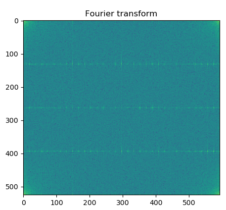
The frequency space image shows several clearly defined vertical and horizontal lines representing the periodic noise we observe in our images. We can test this by setting the magnitude of these frequencies to zero and performing the inverse Fourier analysis returning the original image but without the removed frequencies.
Observing the resulting image, it is clear that the periodic noise of the image is dramatically reduced while maintaining the portions of information we’re actually interested in. Instead of deleting these frequencies from the image we can instead extract them from the image, and perform the inverse transform on these frequencies alone. The resulting image
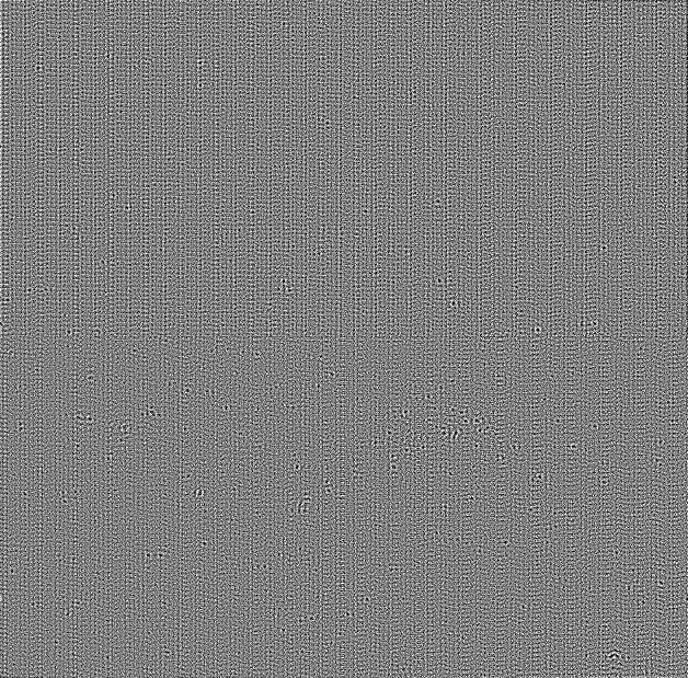 shows the noise texture we extracted from the experimental data.
A noise template is made by saving the output noise image, creating an image of the noise pattern which can be weighted into the simulation images. The result is a simulation image with the same noise as we observe in our experimental data, allowing the algorithm to learn to identify defects with the same noise as our data.
Results
Here are a few samples of the resulting simulation images:
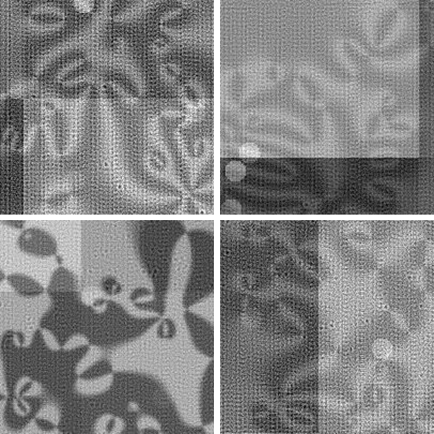
As seen in the images above, there is a great variety of contrast, sharpness, brightness, noise, and brightness shifts throughout the various images.
After training on a set of 1000 noisy simulation images, the model was successfully capable of identifying most major defects present in our experimental data.
